Accelerate SISO Single-Carrier Link Simulation Using GPU
This example shows a comparison of four techniques which can be used to accelerate bit error rate (BER) simulations using System objects in the MATLAB® Communications Toolbox™ software. A small system, based on convolutional coding, illustrates the effect of code generation using the MATLAB® Coder™ product, parallel loop execution using parfor in the Parallel Computing Toolbox™ product, a combination of code generation and parfor, and GPU-based System objects.
The System objects this example features are accessible in the Communications Toolbox product. In order to run this example you must have a MATLAB Coder license, a Parallel Computing Toolbox license, and a sufficient GPU.
System Design and Simulation Parameters
This example uses a simple convolutional coding system to illustrate simulation acceleration strategies. The system generates random message bits using randi. A transmitter encodes these bits using a rate 1/2 convolutional encoder, applies a QPSK modulation scheme, and then transmits the symbols. The symbols pass through an AWGN channel, where signal corruption occurs. QPSK demodulation occurs at the receiver, and the corrupted bits are decoded using the Viterbi algorithm. Finally, the bit error rate is computed. The System objects used in this system are :
comm.ConvolutionalEncoder - convolutional encoding
comm.PSKModulator - QPSK modulation
comm.AWGNChannel - AWGN channel
comm.PSKDemodulator - QPSK demodulation (approx LLR)
comm.ViterbiDecoder - Viterbi decoding
The code for the transceivers can be found in:
Each point along the bit error rate curve represents the result of many iterations of the transceiver code described above. To obtain accurate results in a reasonable amount of time, the simulation will gather at least 200 bit errors per signal-to-noise ratio (SNR) value, and at most 5000 packets of data. A packet represents 2000 message bits. The SNR ranges from 1 dB to 5 dB.
iterCntThreshold = 5000;
minErrThreshold = 200;
msgL = 2000;
snrdb = 1:5;
Initialization
Call the transceiver functions once to factor out setup time and object construction overhead. Objects are stored in persistent variables in each function.
errs  = zeros(length(snrdb),1);
iters = zeros(length(snrdb),1);

berplot = cell(1,5);
numframes = 500; % GPU version runs 500 frames in parallel.

viterbiTransceiverCPU(-10,1,1);
viterbiTransceiverGPU(-10,1,1,numframes);

N=1; % N tracks which simulation variant is run
Workflow
The workflow for this example is:
Run a baseline simulation of System objects
Use MATLAB Coder to generate a MEX function for the simulation
Use parfor to run the bit error rate simulation in parallel
Combine the generated MEX function with parfor
Use the GPU-based System objects
fprintf(1,'Bit Error Rate Acceleration Analysis Example\n\n');
Bit Error Rate Acceleration Analysis Example
Baseline Simulation
To establish a reference point for various acceleration strategies, a bit error rate curve is generated using System objects alone. The code for the transceiver is in viterbiTransceiverCPU.m.
fprintf(1,'***Baseline - Standard System object simulation***\n');

% Create random stream for each snrdb simulation
s = RandStream.create('mrg32k3a','NumStreams',1,...
    'CellOutput',true,'NormalTransform','Inversion');
RandStream.setGlobalStream(s{1});

ts = tic;
for ii=1:numel(snrdb)
    fprintf(1,'Iteration number %d, SNR (dB) = %d\n',ii,snrdb(ii));
    [errs(ii),iters(ii)] = viterbiTransceiverCPU( ...
        snrdb(ii),minErrThreshold,iterCntThreshold);
end
ber = errs./ (msgL* iters);
baseTime=toc(ts);
berplot{N} = ber;
desc{N} = 'baseline';
reportResultsCommSysGPU(N,baseTime,baseTime,'Baseline');
***Baseline - Standard System object simulation***
Iteration number 1, SNR (dB) = 1
Iteration number 2, SNR (dB) = 2
Iteration number 3, SNR (dB) = 3
Iteration number 4, SNR (dB) = 4
Iteration number 5, SNR (dB) = 5
----------------------------------------------------------------------------------------------
Versions of the Transceiver                         | Elapsed Time (sec)| Acceleration Ratio
1. Baseline                                         |           17.9850 |       1.0000
----------------------------------------------------------------------------------------------
Code Generation
Using MATLAB Coder, a MEX file can be generated with optimized C code that matches the precompiled MATLAB code. Because the viterbiTransceiverCPU function conforms to the MATLAB code generation subset, it can be compiled into a MEX function without modification.
You must have a MATLAB Coder license to run this portion of the example.
fprintf(1,'\n***Baseline + codegen***\n');
N=N+1; % Increase simulation counter

% Create the coder object and turn off checks which will cause low
% performance.
fprintf(1,'Generating Code ...');
config_obj = coder.config('MEX');
config_obj.EnableDebugging = false;
config_obj.IntegrityChecks = false;
config_obj.ResponsivenessChecks = false;
config_obj.EchoExpressions = false;

% Generate a MEX file
codegen('viterbiTransceiverCPU.m','-config','config_obj','-args', ...
    {snrdb(1),minErrThreshold,iterCntThreshold} )
fprintf(1,'  Done.\n');

% Run once to eliminate startup overhead.
viterbiTransceiverCPU_mex(-10,1,1);

s = RandStream.getGlobalStream;
reset(s);

% Use the generated MEX function viterbiTransceiverCPU_mex in the
% simulation loop.
ts = tic;
for ii=1:numel(snrdb)
    fprintf(1,'Iteration number %d, SNR (dB) = %d\n',ii,snrdb(ii));
    [errs(ii),iters(ii)] = viterbiTransceiverCPU_mex( ...
        snrdb(ii),minErrThreshold,iterCntThreshold);
end
ber = errs./ (msgL* iters);
trialtime=toc(ts);
berplot{N} = ber;
desc{N} = 'codegen';
reportResultsCommSysGPU(N,trialtime,baseTime,'Baseline + codegen');
***Baseline + codegen***
Generating Code ...Code generation successful.

  Done.
Iteration number 1, SNR (dB) = 1
Iteration number 2, SNR (dB) = 2
Iteration number 3, SNR (dB) = 3
Iteration number 4, SNR (dB) = 4
Iteration number 5, SNR (dB) = 5
----------------------------------------------------------------------------------------------
Versions of the Transceiver                         | Elapsed Time (sec)| Acceleration Ratio
1. Baseline                                         |           17.9850 |       1.0000
2. Baseline + codegen                               |           14.1611 |       1.2700
----------------------------------------------------------------------------------------------
Parfor - Parallel Loop Execution
Using parfor, MATLAB executes the transceiver code against all SNR values in parallel. This requires opening the parallel pool and adding a parfor loop.
You must have a Parallel Computing Toolbox license to run this portion of the example.
fprintf(1,'\n***Baseline + parfor***\n');
fprintf(1,'Accessing multiple CPU cores ...\n');
if isempty(gcp('nocreate'))
    pool = parpool;
    poolWasOpen = false;
else
    pool = gcp;
    poolWasOpen = true;
end
nW=pool.NumWorkers;
N=N+1; % Increase simulation counter

snrN = numel(snrdb);

mT = minErrThreshold / nW;
iT = iterCntThreshold / nW;

errN =  zeros(nW,snrN);
itrN =  zeros(nW,snrN);

% Replicate snrdb
snrdb_rep=repmat(snrdb,nW,1);

% Create an independent stream for each worker
s = RandStream.create('mrg32k3a','NumStreams',nW,...
    'CellOutput',true,'NormalTransform','Inversion');

% Pre-run
parfor jj=1:nW
    RandStream.setGlobalStream(s{jj});
    viterbiTransceiverCPU(-10,1,1);
end

fprintf(1,'Start parfor job ... ');
ts = tic;
parfor jj=1:nW
    for ii=1:snrN
        [err, itr] = viterbiTransceiverCPU(snrdb_rep(jj,ii),mT,iT);
        errN(jj,ii) = err;
        itrN(jj,ii) = itr;
    end
end
ber = sum(errN)./ (msgL*sum(itrN));
trialtime=toc(ts);
fprintf(1,'Done.\n');
berplot{N} = ber;
desc{N} = 'parfor';
reportResultsCommSysGPU(N,trialtime,baseTime,'Baseline + parfor');
***Baseline + parfor***
Accessing multiple CPU cores ...
Starting parallel pool (parpool) using the 'Processes' profile ...
14-Dec-2023 16:59:17: Connected to 3 of 6 parallel pool workers.
Connected to parallel pool with 6 workers.
Start parfor job ... Done.
----------------------------------------------------------------------------------------------
Versions of the Transceiver                         | Elapsed Time (sec)| Acceleration Ratio
1. Baseline                                         |           17.9850 |       1.0000
2. Baseline + codegen                               |           14.1611 |       1.2700
3. Baseline + parfor                                |            4.4148 |       4.0738
----------------------------------------------------------------------------------------------
Parfor and Code Generation
You can combine the last two techniques for additional acceleration. The compiled MEX function can be executed inside of a parfor loop.
You must have a MATLAB Coder license and a Parallel Computing Toolbox license to run this portion of the example.
fprintf(1,'\n***Baseline + codegen + parfor***\n');
N=N+1; % Increase simulation counter

% Pre-run
parfor jj=1:nW
    RandStream.setGlobalStream(s{jj});
    viterbiTransceiverCPU_mex(1,1,1); % use the same mex file
end

fprintf(1,'Start parfor job ... ');
ts = tic;
parfor jj=1:nW
    for ii=1:snrN
        [err, itr] = viterbiTransceiverCPU_mex(snrdb_rep(jj,ii),mT,iT);
        errN(jj,ii) = err;
        itrN(jj,ii) = itr;
    end
end
ber = sum(errN)./ (msgL*sum(itrN));
trialtime=toc(ts);
fprintf(1,'Done.\n');
berplot{N} = ber;
desc{N} = 'codegen + parfor';
reportResultsCommSysGPU(N,trialtime,baseTime, ...
    'Baseline + codegen + parfor');
***Baseline + codegen + parfor***
Start parfor job ... Done.
----------------------------------------------------------------------------------------------
Versions of the Transceiver                         | Elapsed Time (sec)| Acceleration Ratio
1. Baseline                                         |           17.9850 |       1.0000
2. Baseline + codegen                               |           14.1611 |       1.2700
3. Baseline + parfor                                |            4.4148 |       4.0738
4. Baseline + codegen + parfor                      |            3.3120 |       5.4302
----------------------------------------------------------------------------------------------
GPU
The System objects that the viterbiTransceiverCPU function uses are available for execution on the GPU. The GPU-based versions are:
comm.gpu.ConvolutionalEncoder - convolutional encoding
comm.gpu.PSKModulator - QPSK modulation
comm.gpu.AWGNChannel - AWGN channel
comm.gpu.PSKDemodulator - QPSK demodulation (approx LLR)
comm.gpu.ViterbiDecoder - Viterbi decoding
A GPU is most effective when processing large quantities of data at once. The GPU-based System objects can processes multiple frames in a single call to the step method. The numframes variable represents the number of frames processed per call. This is analogous to parfor except that the parallelism is on a per object basis, rather than a per viterbiTransceiverCPU call basis.
You must have a Parallel Computing Toolbox license and a supported GPU device to run this portion of the example. For information on supported devices, see GPU Computing Requirements (Parallel Computing Toolbox).
fprintf(1,'\n***GPU***\n');
N=N+1; %Increase simulation counter

try
    dev = parallel.gpu.GPUDevice.current;
    fprintf(...
        'GPU detected (%s, %d multiprocessors, Compute Capability %s)\n',...
        dev.Name,dev.MultiprocessorCount,dev.ComputeCapability);

    sg = parallel.gpu.RandStream.create('mrg32k3a', ...
        'NumStreams',1,'NormalTransform','Inversion');
    parallel.gpu.RandStream.setGlobalStream(sg);

    ts = tic;
    for ii=1:numel(snrdb)
        fprintf(1,'Iteration number %d, SNR (dB) = %d\n',ii, snrdb(ii));
        [errs(ii),iters(ii)] =viterbiTransceiverGPU( ...
            snrdb(ii),minErrThreshold,iterCntThreshold,numframes);
    end
    ber = errs./ (msgL* iters);
    trialtime=toc(ts);
    berplot{N} = ber;
    desc{N} = 'GPU';
    reportResultsCommSysGPU(N,trialtime,baseTime,'Baseline + GPU');

    fprintf(1,'  Done.\n');

catch %#ok<CTCH>

    % Report that the appropriate GPU was not found.
    fprintf(1, ['Could not find an appropriate GPU or could not ', ...
        'execute GPU code.\n']);

end
***GPU***
GPU detected (Quadro P620, 4 multiprocessors, Compute Capability 6.1)
Iteration number 1, SNR (dB) = 1
Iteration number 2, SNR (dB) = 2
Iteration number 3, SNR (dB) = 3
Iteration number 4, SNR (dB) = 4
Iteration number 5, SNR (dB) = 5
----------------------------------------------------------------------------------------------
Versions of the Transceiver                         | Elapsed Time (sec)| Acceleration Ratio
1. Baseline                                         |           17.9850 |       1.0000
2. Baseline + codegen                               |           14.1611 |       1.2700
3. Baseline + parfor                                |            4.4148 |       4.0738
4. Baseline + codegen + parfor                      |            3.3120 |       5.4302
5. Baseline + GPU                                   |            3.0243 |       5.9469
----------------------------------------------------------------------------------------------
  Done.
Analysis
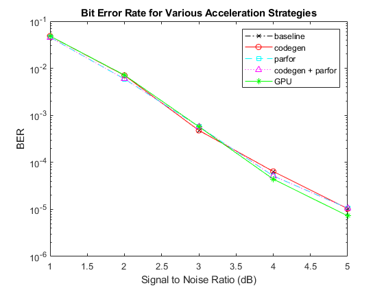
Comparing the results of these trials, it is clear that the GPU is significantly faster than any other simulation acceleration technique. This performance boost requires a very modest change to the simulation code. However, there is no loss in bit error rate performance as the following plot illustrates. The very slight differences in the curves are a result of different random number generation algorithms and/or effects of averaging different quantities of data for the same point on the curve.
lines = {'kx-.','ro-','cs--','m^:','g*-'};
for ii=1:numel(desc)
    semilogy(snrdb,berplot{ii},lines{ii});
    hold on;
end
hold off;
title('Bit Error Rate for Various Acceleration Strategies');
xlabel('Signal to Noise Ratio (dB)');
ylabel('BER');
legend(desc{:});
Cleanup
Leave the parallel pool in the original state.
if ~poolWasOpen
    delete(gcp);
end
Parallel pool using the 'Processes' profile is shutting down.
You can also select a web site from the following list:
Americas
- América Latina (Español)
- Canada (English)
- United States (English)
Europe
- Belgium (English)
- Denmark (English)
- Deutschland (Deutsch)
- España (Español)
- Finland (English)
- France (Français)
- Ireland (English)
- Italia (Italiano)
- Luxembourg (English)
- Netherlands (English)
- Norway (English)
- Österreich (Deutsch)
- Portugal (English)
- Sweden (English)
- Switzerland
- United Kingdom (English)