Multipath Fading Channel
This example shows how to use Rayleigh and Rician multipath fading channel System objects and their built-in visualization to model a fading channel and display the spectral characteristics of the channel. Rayleigh and Rician fading channels are useful models of real-world phenomena in wireless communication. These phenomena include multipath scattering effects, time dispersion, and Doppler shifts that arise from relative motion between the transmitter and receiver.
Processing a signal using a fading channel involves the following steps:
Create a channel System object™ that describes the channel that you want to use. A channel object is a type of MATLAB® variable that contains information about the channel, such as the maximum Doppler shift.
Adjust properties of the System object, as needed to model your channel. For example, you can change the path delays or average path gains.
Call the channel System object like a function to apply the channel model, which generates random discrete path gains and filters the input signal.
Initialization
The following variables control both the Rayleigh and Rician channel objects. By default, the channel is modeled as four fading paths, each representing a cluster of multipath components received at around the same delay.
sampleRate500KHz = 500e3;    % Sample rate of 500 KHz
sampleRate20KHz  = 20e3;     % Sample rate of 20 KHz
maxDopplerShift  = 200; % Max Doppler shift of diffuse components (Hz)
delayVector = (0:5:15)*1e-6; % Discrete delays of four-path channel (s)
gainVector  = [0 -3 -6 -9];  % Average path gains (dB)
The maximum Doppler shift is computed as , where is the mobile speed, f is the carrier frequency, and c is the speed of light. For example, a maximum Doppler shift of 200 Hz (as above) corresponds to a mobile speed of 65 mph (30 m/s) and a carrier frequency of 2 GHz.
By convention, the delay of the first path is typically set to zero. For subsequent paths, a 1 microsecond delay corresponds to a 300 m difference in path length. In some outdoor multipath environments, reflected paths can be up to several kilometers longer than the shortest path. With the path delays specified above, the last path is 4.5 Km longer than the shortest path, and thus arrives 15 microseconds later.
Together, the path delays and path gains specify the average delay profile of the channel. Typically, the average path gains decay exponentially with delay (dB values decay linearly), but the specific delay profile depends on the propagation environment. In the delay profile specified above, we assume a 3 dB decrease in average power for every 5 microseconds of path delay.
The following variables control the Rician channel System object. The Doppler shift of the specular component is typically smaller than the maximum Doppler shift (above) and depends on the direction of travel of the mobile relative to the direction of the specular component. The K-factor specifies the linear ratio of average received power from the specular component relative to that of the associated diffuse components.
KFactor = 10;           % Linear ratio of specular to diffuse power
specDopplerShift = 100; % Doppler shift of specular component (Hz)
Create Channel System Objects
Create comm.RayleighChannel and comm.RicianChannel System objects using the variables defined above. Configure the objects to use their self-contained random stream with a specified seed for path gain generation.
rayChan = comm.RayleighChannel( ...
    SampleRate=sampleRate500KHz, ...
    PathDelays=delayVector, ...
    AveragePathGains=gainVector, ...
    MaximumDopplerShift=maxDopplerShift, ...
    RandomStream="mt19937ar with seed", ...
    Seed=10, ...
    PathGainsOutputPort=true);

ricChan = comm.RicianChannel( ...
    SampleRate=sampleRate500KHz, ...
    PathDelays=delayVector, ...
    AveragePathGains=gainVector, ...
    KFactor=KFactor, ...
    DirectPathDopplerShift=specDopplerShift, ...
    MaximumDopplerShift=maxDopplerShift, ...
    RandomStream="mt19937ar with seed", ...
    Seed=100, ...
    PathGainsOutputPort=true);
Modulation and Channel Filtering
Generate a frame of signal data by using the randi function. In the code here, a frame refers to a vector of information bits. Specify the number of bits transmitted per frame to be 1000. For QPSK modulation, this corresponds to 500 symbols per frame. QPSK-modulate the frame of data, specifying phase offset and bit input, by using the pskmod function. Apply Rayleigh and Rician channel filtering to the modulated data without visualizing the data.
M = 4;               % QPSK modulation
phaseoffset = pi/4;  % Phase offset for QPSK
bitsPerFrame = 1000;
msg = randi([0 1],bitsPerFrame,1);

modSignal = pskmod(msg,M,phaseoffset,InputType='bit');
rayChan(modSignal);
ricChan(modSignal);
Visualization of Channel Response
The fading channel System objects have built-in visualization to show the channel impulse response, frequency response, or Doppler spectrum when the object runs. To invoke it, set the Visualization property to the desired value before calling the object. To reconfigure the Rayleigh and Rician channel System objects release the objects, and then change their property values.
release(rayChan);
release(ricChan);
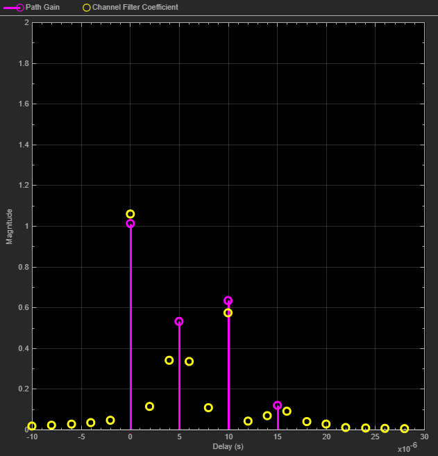
Setting the Visualization property to "Impulse response" shows the bandlimited impulse response (yellow circles). The visualization also shows the delays and magnitudes of the underlying fading path gains (pink stembars) clustered around the peak of the impulse response. Note that the path gains do not equal the AveragePathGains property value because the Doppler effect causes the gains to fluctuate over time.
Similarly, setting the Visualization property to "Frequency response" shows the frequency response (DFT transformation) of the impulses. You can also set Visualization to "Impulse and frequency responses" to display both impulse and frequency responses side by side.
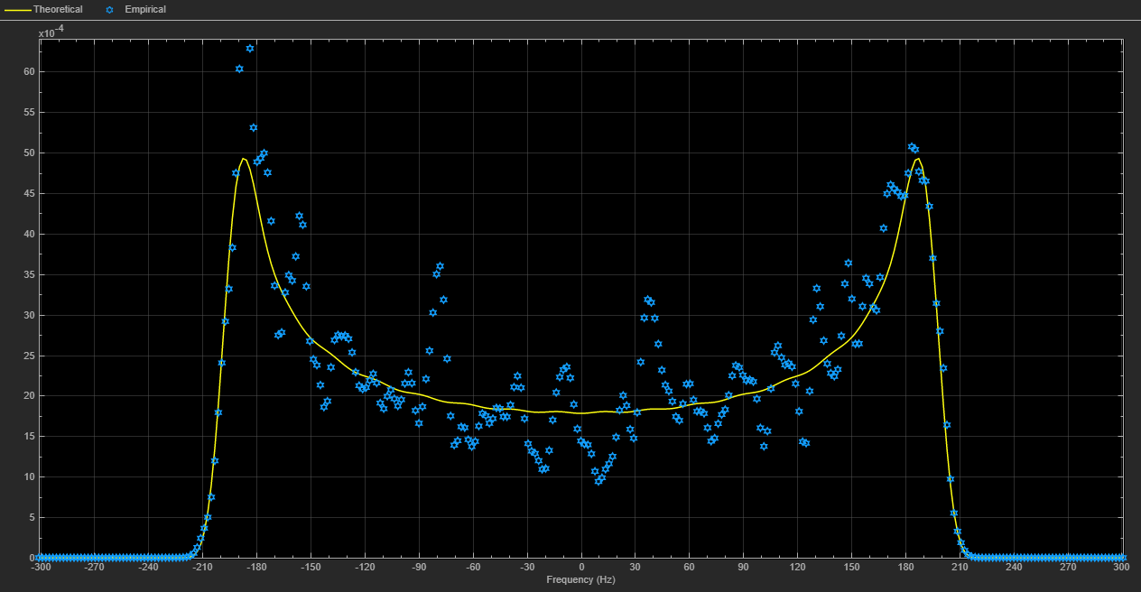
Setting the Visualization property to "Doppler spectrum" shows the Doppler spectrum for the first discrete path, which is a statistical characterization of the fading process. Instantaneous empirical measurements are plotted of the Doppler spectrum (blue stars). Over time with more samples processed, the average of this measurement better approximates the theoretical Doppler spectrum (yellow curve).
Visualization settings allow you to tradeoff between optimal plot accuracy and simulation speed. The SamplesToDisplay property controls the percentage of the input samples to be visualized. In general, the smaller the percentage, the faster the simulation runs. If you want to see the channel response for every input sample, set SamplesToDisplay to "100%", but this leads to longer simulation run time and is typically not necessary for representative signal plots.
Wideband or Frequency-Selective Fading
Display the impulse and frequency response of the QPSK-modulated signal after Rayleigh fading. The channel frequency response is not flat and may have deep fades over the 500 KHz bandwidth. Because the power level varies over the bandwidth of the signal, it is referred to as wideband or frequency-selective fading.
rayChan.Visualization = "Impulse and frequency responses";
rayChan.SamplesToDisplay = "100%";
% Display impulse and frequency responses for 2 frames
numFrames = 2;
for i = 1:numFrames
    % Create random data
    msg = randi([0 1],bitsPerFrame,1);
    % Modulate data
    modSignal = pskmod(msg,M,phaseoffset,InputType='bit');
    % Filter data through channel and show channel responses
    rayChan(modSignal);
end
Display a statistical characterization of the fading process for the same channel specification by releasing the Rayleigh channel object and reconfiguring the object to display the Doppler spectrum for its first discrete path.
release(rayChan);
rayChan.Visualization = "Doppler spectrum";

% Display Doppler spectrum from 5000 frame transmission
numFrames = 5000;
for i = 1:numFrames
    msg = randi([0 1],bitsPerFrame,1);
    modSignal = pskmod(msg,M,phaseoffset,InputType='bit');
    rayChan(modSignal);
end
Narrowband or Frequency-Flat Fading
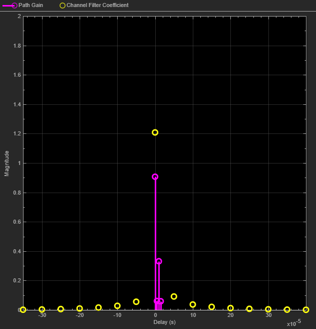
When the bandwidth is too small for the signal to resolve the individual components, the frequency response is approximately flat because of the minimal time dispersion caused by the multipath channel. This kind of multipath fading is often referred to as narrowband fading, or frequency-flat fading.
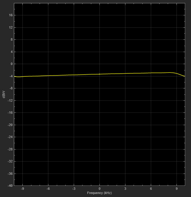
Reduce the signal bandwidth from 500 Kb/s (250 Ksym/s) to 20 Kb/s (10 Ksym/s), so the delay span (15 microseconds) of the channel is much smaller than the QPSK symbol period (100 microseconds). The resultant impulse response has very small intersymbol interference (ISI) and the frequency response is approximately flat.
release(rayChan);
rayChan.Visualization = "Impulse and frequency responses";
rayChan.SampleRate = sampleRate20KHz;
rayChan.SamplesToDisplay = "25%";  % Display one of every four samples

% Display impulse and frequency responses for 2 frames
numFrames = 2;
for i = 1:numFrames
    msg = randi([0 1],bitsPerFrame,1);
    modSignal = pskmod(msg,M,phaseoffset,InputType='bit');
    rayChan(modSignal);
end
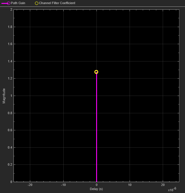
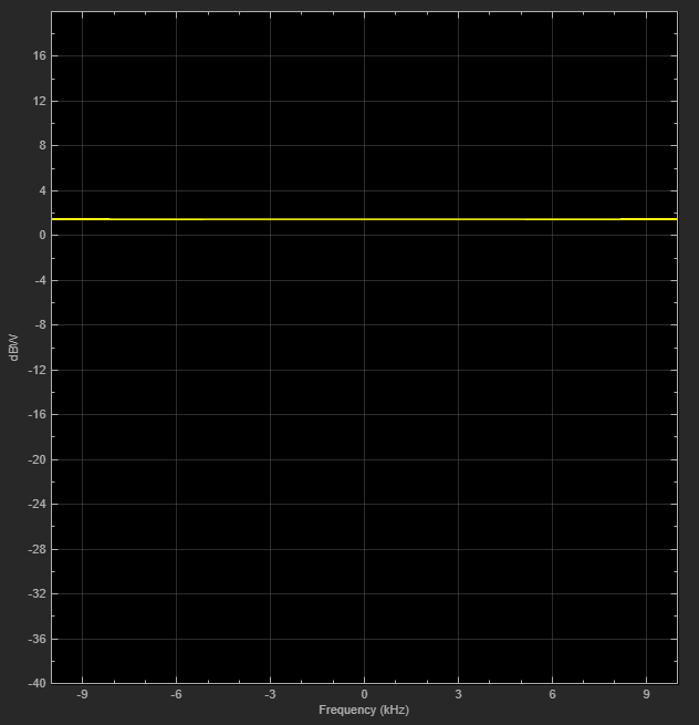
For narrowband fading channels, a single-path fading model can accurately represent the channel. To simplify and speed up simulations when the channel has narrowband fading, consider replacing a multipath fading model with a single-path fading model. The following settings correspond to a narrowband fading channel and, as shown by the plot, the frequency response is completely flat.
release(rayChan);
rayChan.PathDelays = 0;        % Single fading path with zero delay
rayChan.AveragePathGains = 0;  % Average path gain of 1 (0 dB)
Display impulse and frequency responses for 2 frames.
for i = 1:numFrames
    msg = randi([0 1],bitsPerFrame,1);
    modSignal = pskmod(msg,M,phaseoffset,InputType='bit');
    rayChan(modSignal);
end
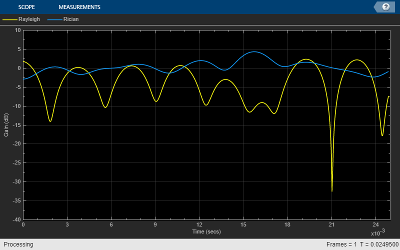
The Rician fading channel System object models line-of-sight propagation in addition to diffuse multipath scattering. This results in a smaller variation in the magnitude of path gains. To compare the variation between Rayleigh and Rician channels, view their path gains over time by using a timescope object.
Observe the magnitude fluctuates over approximately a 10 dB range for the Rician fading channel (blue curve), compared with 30-40 dB for the Rayleigh fading channel (yellow curve). For the Rician fading channel, this variation would be further reduced by increasing the K-factor (currently set to 10).
release(rayChan);
rayChan.Visualization = "Off"; % Turn off Rayliegh object visualization
ricChan.Visualization = "Off"; % Turn off Rician object visualization

% Same sample rate and delay profile for the Rayleigh and Rician objects
ricChan.SampleRate = rayChan.SampleRate;
ricChan.PathDelays = rayChan.PathDelays;
ricChan.AveragePathGains = rayChan.AveragePathGains;

% Configure a Time Scope System object to show path gain magnitude
gainScope = timescope( ...
    SampleRate=rayChan.SampleRate, ...
    TimeSpanSource="Property",...
    TimeSpan=bitsPerFrame/2/rayChan.SampleRate, ... % One frame span
    Name="Multipath Gain", ...
    ChannelName=["Rayleigh","Rician"], ...
    ShowGrid=true, ...
    YLimits=[-40 10], ...
    YLabel="Gain (dB)");

% Compare the path gain outputs from both objects for one frame
msg = randi([0 1],bitsPerFrame,1);
modSignal = pskmod(msg,M,phaseoffset,InputType='bit');
[~,rayPathGain] = rayChan(modSignal);
[~,ricPathGain] = ricChan(modSignal);
% Form the path gains as a two-channel input to the time scope
gainScope(10*log10(abs([rayPathGain,ricPathGain]).^2));
Fading Channel Impact on Signal Constellation
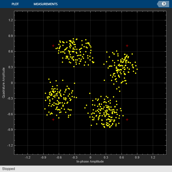
Return to the original four-path Rayleigh fading channel and show the impact of narrowband fading on the signal constellation by using a comm.ConstellationDiagram System object. To slow down the channel dynamics for visualization purposes, we reduce the maximum Doppler shift to 5 Hz. Compared with the QPSK channel input signal, you can observe signal attenuation and rotation at the channel output, as well as some signal distortion due to the small amount of ISI in the received signal.
release(rayChan);

rayChan.PathDelays = delayVector;
rayChan.AveragePathGains = gainVector;
rayChan.MaximumDopplerShift = 5;

constDiag = comm.ConstellationDiagram( ...
    Name="Received Signal After Rayleigh Fading");

numFrames = 16;
for n = 1:numFrames
    msg = randi([0 1],bitsPerFrame,1);
    modSignal = pskmod(msg,M,phaseoffset,InputType='bit');
    rayChanOut = rayChan(modSignal);
    constDiag(rayChanOut);
end
release(rayChan);
release(constDiag);
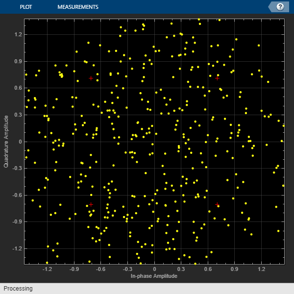
Adjust the Rayliegh channel sample rate back to 500 KHz. This increases the signal bandwidth to 500 Kb/s, which corresponds to 250 Ksym/s for the QPSK-modulated signal. Replot the constellation diagram to observe much greater distortion in the signal constellation due to the ISI associated with the time dispersion of the wideband signal. The delay span (15 microseconds) of the channel is now larger than the QPSK symbol period (4 microseconds), so the resultant bandlimited impulse response is no longer approximately flat.
rayChan.SampleRate = sampleRate500KHz;

for n = 1:numFrames
    msg = randi([0 1],bitsPerFrame,1);
    modSignal = pskmod(msg,M,phaseoffset,InputType='bit');
    rayChanOut = rayChan(modSignal);
    constDiag(rayChanOut);
end
You can also select a web site from the following list:
Americas
- América Latina (Español)
- Canada (English)
- United States (English)
Europe
- Belgium (English)
- Denmark (English)
- Deutschland (Deutsch)
- España (Español)
- Finland (English)
- France (Français)
- Ireland (English)
- Italia (Italiano)
- Luxembourg (English)
- Netherlands (English)
- Norway (English)
- Österreich (Deutsch)
- Portugal (English)
- Sweden (English)
- Switzerland
- United Kingdom (English)