Digit Classification Using HOG Features
This example shows how to classify digits using HOG features and a multiclass SVM classifier.
Object classification is an important task in many computer vision applications, including surveillance, automotive safety, and image retrieval. For example, in an automotive safety application, you may need to classify nearby objects as pedestrians or vehicles. Regardless of the type of object being classified, the basic procedure for creating an object classifier is:
Acquire a labeled data set with images of the desired object.
Partition the data set into a training set and a test set.
Train the classifier using features extracted from the training set.
Test the classifier using features extracted from the test set.
To illustrate, this example shows how to classify numerical digits using HOG (Histogram of Oriented Gradient) features [1] and a multiclass SVM (Support Vector Machine) classifier. This type of classification is often used in many Optical Character Recognition (OCR) applications.
The example uses the fitcecoc function from the Statistics and Machine Learning Toolbox™ and the extractHOGFeatures function from the Computer Vision Toolbox™.
Digit Data Set
Synthetic digit images are used for training. The training images each contain a digit surrounded by other digits, which mimics how digits are normally seen together. Using synthetic images is convenient and it enables the creation of a variety of training samples without having to manually collect them. For testing, scans of handwritten digits are used to validate how well the classifier performs on data that is different than the training data. Although this is not the most representative data set, there is enough data to train and test a classifier, and show the feasibility of the approach.
% Load training and test data using |imageDatastore|.
syntheticDir   = fullfile(toolboxdir('vision'),'visiondata','digits','synthetic');
handwrittenDir = fullfile(toolboxdir('vision'),'visiondata','digits','handwritten');

% |imageDatastore| recursively scans the directory tree containing the
% images. Folder names are automatically used as labels for each image.
trainingSet = imageDatastore(syntheticDir,'IncludeSubfolders',true,'LabelSource','foldernames');
testSet     = imageDatastore(handwrittenDir,'IncludeSubfolders',true,'LabelSource','foldernames');
Use countEachLabel to tabulate the number of images associated with each label. In this example, the training set consists of 101 images for each of the 10 digits. The test set consists of 12 images per digit.
countEachLabel(trainingSet)
ans=10×2 table
    Label    Count
    _____    _____

      0       101
      1       101
      2       101
      3       101
      4       101
      5       101
      6       101
      7       101
      8       101
      9       101
countEachLabel(testSet)
ans=10×2 table
    Label    Count
    _____    _____

      0       12
      1       12
      2       12
      3       12
      4       12
      5       12
      6       12
      7       12
      8       12
      9       12
Show a few of the training and test images
figure;

subplot(2,3,1);
imshow(trainingSet.Files{102});

subplot(2,3,2);
imshow(trainingSet.Files{304});

subplot(2,3,3);
imshow(trainingSet.Files{809});

subplot(2,3,4);
imshow(testSet.Files{13});

subplot(2,3,5);
imshow(testSet.Files{37});

subplot(2,3,6);
imshow(testSet.Files{97});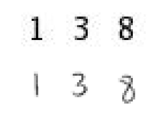
Prior to training and testing a classifier, a pre-processing step is applied to remove noise artifacts introduced while collecting the image samples. This provides better feature vectors for training the classifier.
% Show pre-processing results
exTestImage = readimage(testSet,37);
processedImage = imbinarize(im2gray(exTestImage));

figure;

subplot(1,2,1)
imshow(exTestImage)

subplot(1,2,2)
imshow(processedImage)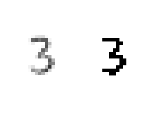
Using HOG Features
The data used to train the classifier are HOG feature vectors extracted from the training images. Therefore, it is important to make sure the HOG feature vector encodes the right amount of information about the object. The extractHOGFeatures function returns a visualization output that can help form some intuition about just what the "right amount of information" means. By varying the HOG cell size parameter and visualizing the result, you can see the effect the cell size parameter has on the amount of shape information encoded in the feature vector:
img = readimage(trainingSet, 206);

% Extract HOG features and HOG visualization
[hog_2x2, vis2x2] = extractHOGFeatures(img,'CellSize',[2 2]);
[hog_4x4, vis4x4] = extractHOGFeatures(img,'CellSize',[4 4]);
[hog_8x8, vis8x8] = extractHOGFeatures(img,'CellSize',[8 8]);

% Show the original image
figure;
subplot(2,3,1:3); imshow(img);

% Visualize the HOG features
subplot(2,3,4);
plot(vis2x2);
title({'CellSize = [2 2]'; ['Length = ' num2str(length(hog_2x2))]});

subplot(2,3,5);
plot(vis4x4);
title({'CellSize = [4 4]'; ['Length = ' num2str(length(hog_4x4))]});

subplot(2,3,6);
plot(vis8x8);
title({'CellSize = [8 8]'; ['Length = ' num2str(length(hog_8x8))]});
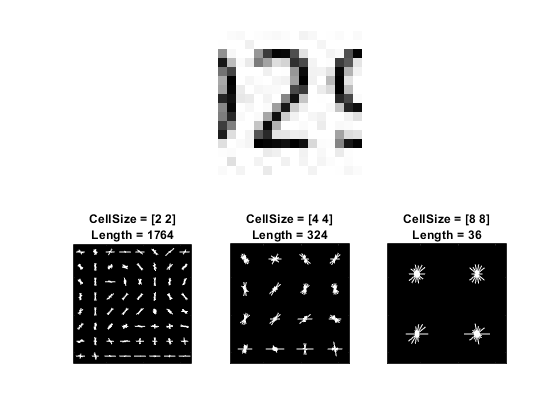
The visualization shows that a cell size of [8 8] does not encode much shape information, while a cell size of [2 2] encodes a lot of shape information but increases the dimensionality of the HOG feature vector significantly. A good compromise is a 4-by-4 cell size. This size setting encodes enough spatial information to visually identify a digit shape while limiting the number of dimensions in the HOG feature vector, which helps speed up training. In practice, the HOG parameters should be varied with repeated classifier training and testing to identify the optimal parameter settings.
cellSize = [4 4];
hogFeatureSize = length(hog_4x4);
Train a Digit Classifier
Digit classification is a multiclass classification problem, where you have to classify an image into one out of the ten possible digit classes. In this example, the fitcecoc function from the Statistics and Machine Learning Toolbox™ is used to create a multiclass classifier using binary SVMs.
Start by extracting HOG features from the training set. These features will be used to train the classifier.
% Loop over the trainingSet and extract HOG features from each image. A
% similar procedure will be used to extract features from the testSet.

numImages = numel(trainingSet.Files);
trainingFeatures = zeros(numImages,hogFeatureSize,'single');

for i = 1:numImages
    img = readimage(trainingSet,i);

    img = im2gray(img);

    % Apply pre-processing steps
    img = imbinarize(img);

    trainingFeatures(i, :) = extractHOGFeatures(img,'CellSize',cellSize);
end

% Get labels for each image.
trainingLabels = trainingSet.Labels;
Next, train a classifier using the extracted features.
% fitcecoc uses SVM learners and a 'One-vs-One' encoding scheme.
classifier = fitcecoc(trainingFeatures, trainingLabels);
Evaluate the Digit Classifier
Evaluate the digit classifier using images from the test set, and generate a confusion matrix to quantify the classifier accuracy.
As in the training step, first extract HOG features from the test images. These features will be used to make predictions using the trained classifier.
% Extract HOG features from the test set. The procedure is similar to what
% was shown earlier and is encapsulated as a helper function for brevity.
[testFeatures, testLabels] = helperExtractHOGFeaturesFromImageSet(testSet, hogFeatureSize, cellSize);

% Make class predictions using the test features.
predictedLabels = predict(classifier, testFeatures);

% Tabulate the results using a confusion matrix.
confMat = confusionmat(testLabels, predictedLabels);

helperDisplayConfusionMatrix(confMat)
digit  | 0        1        2        3        4        5        6        7        8        9
---------------------------------------------------------------------------------------------------
0      | 0.25     0.00     0.08     0.00     0.00     0.00     0.58     0.00     0.08     0.00
1      | 0.00     0.75     0.00     0.00     0.08     0.00     0.00     0.08     0.08     0.00
2      | 0.00     0.00     0.67     0.17     0.00     0.00     0.08     0.00     0.00     0.08
3      | 0.00     0.00     0.00     0.58     0.00     0.00     0.33     0.00     0.00     0.08
4      | 0.00     0.08     0.00     0.17     0.75     0.00     0.00     0.00     0.00     0.00
5      | 0.00     0.00     0.00     0.00     0.00     0.33     0.58     0.00     0.08     0.00
6      | 0.00     0.00     0.00     0.00     0.25     0.00     0.67     0.00     0.08     0.00
7      | 0.00     0.08     0.08     0.33     0.00     0.00     0.17     0.25     0.00     0.08
8      | 0.00     0.00     0.00     0.08     0.00     0.00     0.00     0.08     0.67     0.17
9      | 0.00     0.08     0.00     0.25     0.17     0.00     0.08     0.00     0.00     0.42
The table shows the confusion matrix in percentage form. The columns of the matrix represent the predicted labels, while the rows represent the known labels. For this test set, digit 0 is often misclassified as 6, most likely due to their similar shapes. Similar errors are seen for 9 and 3. Training with a more representative data set like MNIST [2] or SVHN [3], which contain thousands of handwritten characters, is likely to produce a better classifier compared with the one created using this synthetic data set.
Summary
This example illustrated the basic procedure for creating a multiclass object classifier using the extractHOGfeatures function from the Computer Vision Toolbox and the fitcecoc function from the Statistics and Machine Learning Toolbox™. Although HOG features and an ECOC classifier were used here, other features and machine learning algorithms can be used in the same way. For instance, you can explore using different feature types for training the classifier; or you can see the effect of using other machine learning algorithms available in the Statistics and Machine Learning Toolbox™ such as k-nearest neighbors.
Supporting Functions
function helperDisplayConfusionMatrix(confMat)
% Display the confusion matrix in a formatted table.

% Convert confusion matrix into percentage form
confMat = bsxfun(@rdivide,confMat,sum(confMat,2));

digits = '0':'9';
colHeadings = arrayfun(@(x)sprintf('%d',x),0:9,'UniformOutput',false);
format = repmat('%-9s',1,11);
header = sprintf(format,'digit  |',colHeadings{:});
fprintf('\n%s\n%s\n',header,repmat('-',size(header)));
for idx = 1:numel(digits)
    fprintf('%-9s',   [digits(idx) '      |']);
    fprintf('%-9.2f', confMat(idx,:));
    fprintf('\n')
end
end
function [features, setLabels] = helperExtractHOGFeaturesFromImageSet(imds, hogFeatureSize, cellSize)
% Extract HOG features from an imageDatastore.

setLabels = imds.Labels;
numImages = numel(imds.Files);
features  = zeros(numImages,hogFeatureSize,'single');

% Process each image and extract features
for j = 1:numImages
    img = readimage(imds,j);
    img = im2gray(img);

    % Apply pre-processing steps
    img = imbinarize(img);

    features(j, :) = extractHOGFeatures(img,'CellSize',cellSize);
end
end
References
[1] N. Dalal and B. Triggs, "Histograms of Oriented Gradients for Human Detection", Proc. IEEE Conf. Computer Vision and Pattern Recognition, vol. 1, pp. 886-893, 2005.
[2] LeCun, Y., Bottou, L., Bengio, Y., and Haffner, P. (1998). Gradient-based learning applied to document recognition. Proceedings of the IEEE, 86, 2278-2324.
[3] Y. Netzer, T. Wang, A. Coates, A. Bissacco, B. Wu, A.Y. Ng, Reading Digits in Natural Images with Unsupervised Feature Learning NIPS Workshop on Deep Learning and Unsupervised Feature Learning 2011.
Related Topics
You can also select a web site from the following list:
Americas
- América Latina (Español)
- Canada (English)
- United States (English)
Europe
- Belgium (English)
- Denmark (English)
- Deutschland (Deutsch)
- España (Español)
- Finland (English)
- France (Français)
- Ireland (English)
- Italia (Italiano)
- Luxembourg (English)
- Netherlands (English)
- Norway (English)
- Österreich (Deutsch)
- Portugal (English)
- Sweden (English)
- Switzerland
- United Kingdom (English)