Main Content

trainlm

Levenberg-Marquardt backpropagation

Description

net.trainFcn = 'trainlm' sets the network trainFcn property.

example

[trainedNet,tr] = train(net,...) trains the network with trainlm.

trainlm is a network training function that updates weight and bias values according to Levenberg-Marquardt optimization.

trainlm is often the fastest backpropagation algorithm in the toolbox, and is highly recommended as a first-choice supervised algorithm, although it does require more memory than other algorithms.

Training occurs according to trainlm training parameters, shown here with their default values:

  • net.trainParam.epochs — Maximum number of epochs to train. The default value is 1000.

  • net.trainParam.goal — Performance goal. The default value is 0.

  • net.trainParam.max_fail — Maximum validation failures. The default value is 6.

  • net.trainParam.min_grad — Minimum performance gradient. The default value is 1e-7.

  • net.trainParam.mu — Initial mu. The default value is 0.001.

  • net.trainParam.mu_dec — Decrease factor for mu. The default value is 0.1.

  • net.trainParam.mu_inc — Increase factor for mu. The default value is 10.

  • net.trainParam.mu_max — Maximum value for mu. The default value is 1e10.

  • net.trainParam.show — Epochs between displays (NaN for no displays). The default value is 25.

  • net.trainParam.showCommandLine — Generate command-line output. The default value is false.

  • net.trainParam.showWindow — Show training GUI. The default value is true.

  • net.trainParam.time — Maximum time to train in seconds. The default value is inf.

Validation vectors are used to stop training early if the network performance on the validation vectors fails to improve or remains the same for max_fail epochs in a row. Test vectors are used as a further check that the network is generalizing well, but do not have any effect on training.

Examples

collapse all

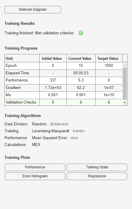
This example shows how to train a neural network using the trainlm train function.

Here a neural network is trained to predict body fat percentages.

[x, t] = bodyfat_dataset;
net = feedforwardnet(10, 'trainlm');
net = train(net, x, t);

Figure Neural Network Training (19-Aug-2023 11:42:44) contains an object of type uigridlayout.

y = net(x);

Input Arguments

collapse all

Input network, specified as a network object. To create a network object, use for example, feedforwardnet or narxnet.

Output Arguments

collapse all

Trained network, returned as a network object.

Training record (epoch and perf), returned as a structure whose fields depend on the network training function (net.NET.trainFcn). It can include fields such as:

  • Training, data division, and performance functions and parameters

  • Data division indices for training, validation and test sets

  • Data division masks for training validation and test sets

  • Number of epochs (num_epochs) and the best epoch (best_epoch).

  • A list of training state names (states).

  • Fields for each state name recording its value throughout training

  • Performances of the best network (best_perf, best_vperf, best_tperf)

Limitations

This function uses the Jacobian for calculations, which assumes that performance is a mean or sum of squared errors. Therefore, networks trained with this function must use either the mse or sse performance function.

More About

collapse all

Levenberg-Marquardt Algorithm

Like the quasi-Newton methods, the Levenberg-Marquardt algorithm was designed to approach second-order training speed without having to compute the Hessian matrix. When the performance function has the form of a sum of squares (as is typical in training feedforward networks), then the Hessian matrix can be approximated as

H = JTJ(1)

and the gradient can be computed as

g = JTe(2)

where J is the Jacobian matrix that contains first derivatives of the network errors with respect to the weights and biases, and e is a vector of network errors. The Jacobian matrix can be computed through a standard backpropagation technique (see [HaMe94]) that is much less complex than computing the Hessian matrix.

The Levenberg-Marquardt algorithm uses this approximation to the Hessian matrix in the following Newton-like update:

xk+1=xk[JTJ+μI]1JTe

When the scalar µ is zero, this is just Newton’s method, using the approximate Hessian matrix. When µ is large, this becomes gradient descent with a small step size. Newton’s method is faster and more accurate near an error minimum, so the aim is to shift toward Newton’s method as quickly as possible. Thus, µ is decreased after each successful step (reduction in performance function) and is increased only when a tentative step would increase the performance function. In this way, the performance function is always reduced at each iteration of the algorithm.

The original description of the Levenberg-Marquardt algorithm is given in [Marq63]. The application of Levenberg-Marquardt to neural network training is described in [HaMe94] and starting on page 12-19 of [HDB96]. This algorithm appears to be the fastest method for training moderate-sized feedforward neural networks (up to several hundred weights). It also has an efficient implementation in MATLAB® software, because the solution of the matrix equation is a built-in function, so its attributes become even more pronounced in a MATLAB environment.

Network Use

You can create a standard network that uses trainlm with feedforwardnet or cascadeforwardnet. To prepare a custom network to be trained with trainlm,

  1. Set NET.trainFcn to trainlm. This sets NET.trainParam to trainlm’s default parameters.

  2. Set NET.trainParam properties to desired values.

In either case, calling train with the resulting network trains the network with trainlm. See feedforwardnet and cascadeforwardnet for examples.

Algorithms

trainlm supports training with validation and test vectors if the network’s NET.divideFcn property is set to a data division function. Validation vectors are used to stop training early if the network performance on the validation vectors fails to improve or remains the same for max_fail epochs in a row. Test vectors are used as a further check that the network is generalizing well, but do not have any effect on training.

trainlm can train any network as long as its weight, net input, and transfer functions have derivative functions.

Backpropagation is used to calculate the Jacobian jX of performance perf with respect to the weight and bias variables X. Each variable is adjusted according to Levenberg-Marquardt,

jj = jX * jX
je = jX * E
dX = -(jj+I*mu) \ je

where E is all errors and I is the identity matrix.

The adaptive value mu is increased by mu_inc until the change above results in a reduced performance value. The change is then made to the network and mu is decreased by mu_dec.

Training stops when any of these conditions occurs:

  • The maximum number of epochs (repetitions) is reached.

  • The maximum amount of time is exceeded.

  • Performance is minimized to the goal.

  • The performance gradient falls below min_grad.

  • mu exceeds mu_max.

  • Validation performance (validation error) has increased more than max_fail times since the last time it decreased (when using validation).

Version History

Introduced before R2006a